Total Offense Score

Total Offense Score

The goal of this article is to create a new metric to judge a single player’s offensive production. I know there is a ton out there already (PER, OWS, OBPM, etc.) but I wanted to try my hand at creating one and possibly find ways improve upon them. My metric will mostly be based on total production and how efficient that player was at achieving that production.

Method

I measured total production as points generated (PGEN), which is the sum of the points the player generated either through scoring or passing, for which we will include second assists and free throw assists. The formula is as follows:

\[PGEN = PTS + \frac{AST\:PTS\:CREATED}{AST + FT\:AST} * (AST + 2nd\:AST + FT\:AST)\]

We are getting our stats from nba.com/stats, which includes FT AST in their calculation for AST PTS CREATED but does not include 2nd AST so we find the player’s points per assist and multiply that by the total of the three types to estimate the total points generated through passing.

To measure efficiency I will be using a stat called Individual Offensive Efficiency with Assist Opportunities (IOEwAO) which is PGEN divided by the number or possessions that player terminated (NPTwAO) either by shooting, making a pass that leads to a shot, or turning the ball over. I know those are complicated abbreviations but IOEwAO can differ from just Individual Offensive Efficiency which doesn’t take into account potential assists. I will be using assist opportunities as it is more indicative of how often that player ends a possession.

\[NPTwAO = FGA + .44*FTA + TOV + ASSIST\:OPPORTUNITIES + 2nd\:AST - OREB\] \[IOEwAO = \frac{PGEN}{NPTwAO}\]

You may notice that I included offensive rebounds in the NPTwAO calculation, this is because NPT stands for net possessions terminated and offensive rebound earns the team another possession. Also, FT AST was not included because on nba.com/stats Assist Opportunities and FT AST overlap.

We multiply free throws by 0.44 since not every time does a player shoot two free throws for a foul. 0.44 gives us a better estimate of the actual number of possessions.

Ok so this is the bulk of the information that will be used, now I have to get the data. Using the nba_api repository on github, I wrote a Python Script to scrape the necessary data for every active player in the 2019-20 NBA season into a spreadsheet, and calculated their PGEN, NPTwAO, and IOEwAO along with some other metrics that this article will not focus on.

import pandas as pd

df = pd.read_csv('offensive_efficiency_19_20.csv')
df[['PLAYER_NAME', 'TEAM_ABBREVIATION', 'GP', 'PTS', 'FGA', 'FTA',
    'TOV', 'OREB', 'PGen', 'NPTwAO', 'PGen/G', 'NPTwAO/G', 'IOEwAO']].head(10)

	PLAYER_NAME	TEAM_ABBREVIATION	GP	PTS	FGA	FTA	TOV	OREB	PGen	NPTwAO	PGen/G	NPTwAO/G	IOEwAO
0	Aaron Gordon	ORL	62	894	767	224	100	107	1501.200000	1296.56	24.212903	21.27	1.157833
1	Aaron Holiday	IND	66	627	563	87	88	22	1287.780876	1133.28	19.511831	17.56	1.136331
2	Abdel Nader	OKC	55	345	263	66	43	14	449.268293	391.04	8.168514	7.16	1.148906
3	Adam Mokoka	CHI	11	32	28	4	2	7	44.500000	33.76	4.045455	3.07	1.318128
4	Admiral Schofield	WAS	33	99	92	15	7	7	143.705882	128.60	4.354724	3.96	1.117464
5	Al Horford	PHI	67	798	709	80	80	103	1512.297945	1156.20	22.571611	17.59	1.307990
6	Al-Farouq Aminu	ORL	18	78	86	29	17	24	137.400000	140.76	7.633333	8.04	0.976130
7	Alec Burks	PHI	66	993	768	265	91	48	1522.879808	1302.60	23.073936	20.02	1.169108
8	Alen Smailagic	GSW	14	59	40	19	11	10	93.000000	66.36	6.642857	4.74	1.401447
9	Alex Caruso	LAL	64	349	291	94	53	17	679.244604	603.36	10.613197	9.66	1.125770

The full spreadsheet contains 41 columns. If you are interested in checking it out, it can be found on my github, but the above columns are what we are going to use in this article.

First let’s find the league average in points per possession. This can be closely estimated by dividing the total points by the total possessions, using the .44 weight for free throws mentioned before.

\[PPP = \frac{PTS}{FGA + .44*FTA + TOV - OREB}\]

ppp = df['PTS'].sum() / (df['FGA'].sum() + .44*df['FTA'].sum() + df['TOV'].sum() - df['OREB'].sum())
print(ppp)

1.0873277667011825

So roughly 1.09 points are scored per possession in the NBA. Having an IOEwAO above this would mean the player produces points at an above average rate, which is good, and should be rewarded in our metric. A below average rate should be punished. To accomplish this, I will take the players PGEN/G and raise it to the power of their IOEwAO divided by PPP which we will call the efficiency factor.

\[PGEN/G^{\frac{IOEwAO}{PPP}}\]

This makes it so a player’s PGEN/G value increases at an exponential rate if it was done on good efficiency, and decreases at an exponential rate on poor efficiency. For example:

print('PGen = 30, IOEwAO = 1, Score =', 30**(1/1.087))
print('PGen = 30, IOEwAO = 1.2, Score =', 30**(1.2/1.087))

PGen = 30, IOEwAO = 1, Score = 22.85057844894064
PGen = 30, IOEwAO = 1.2, Score = 42.724465491574115

Using this, lets see how players stack up against each other. Note that this is a average per game metric which differs from some like OWS and OPBM.

df['Score'] = df['PGen/G'] ** (df['IOEwAO'] / ppp)
df[['PLAYER_NAME', 'NPTwAO/G', 'PGen/G', 'IOEwAO', 'Score']].sort_values('Score', ascending = False).head(25)

	PLAYER_NAME	NPTwAO/G	PGen/G	IOEwAO	Score
90	Damian Lillard	42.07	52.270929	1.261881	98.650533
364	Mitchell Robinson	5.51	11.190416	2.049158	94.762398
215	James Harden	47.50	56.209223	1.200825	85.596552
383	Nikola Jokic	29.51	38.220744	1.324564	84.630986
424	Rudy Gobert	12.11	19.491754	1.621689	83.896069
312	Kyrie Irving	37.89	46.461379	1.254221	83.747851
221	Jarrett Allen	9.21	15.802198	1.734327	81.657820
325	Luka Doncic	45.48	53.628274	1.196849	80.091785
281	Karl-Anthony Towns	29.36	37.659113	1.309635	79.078980
319	LeBron James	44.95	52.825918	1.196271	78.607847
175	Giannis Antetokounmpo	37.82	45.957049	1.225386	74.717450
76	Clint Capela	11.53	18.265734	1.608916	73.593774
245	John Collins	18.46	26.192835	1.426170	72.465101
474	Trae Young	48.45	55.033549	1.158617	71.573127
133	Domantas Sabonis	24.42	31.984065	1.329774	69.262019
33	Ben Simmons	32.90	39.960157	1.235801	66.119093
23	Anthony Davis	28.05	35.397849	1.273747	65.244666
186	Hassan Whiteside	12.41	18.975417	1.542605	65.070609
42	Bradley Beal	41.69	47.880432	1.169778	64.203828
239	Jimmy Butler	30.16	36.820908	1.253294	63.846615
110	DeMar DeRozan	31.95	38.943015	1.230290	63.028871
444	Stephen Curry	35.49	41.270000	1.210690	62.941262
125	Devin Booker	39.49	45.710849	1.177698	62.804072
31	Bam Adebayo	23.29	30.257050	1.319444	62.653395
282	Kawhi Leonard	35.24	41.560621	1.199544	61.057069

This is the top 25 players ranked by our new score.

Our current formula would tell us that last year, Mitchell Robinson was one of the most productive offensive players in the league. It’s understandable if you don’t believe this, but he did have a superb IOEwAO at 2.005, much better than the rest of the top 25. However, if you notice, he only had about 5.5 possessions terminated a game so it was much easier to reach his high efficiency compared to the number 1 player, Damian Lillard, who had 42 possessions terminated per game.

This is a flaw that we need to account for. To do this I will introduce another equation and variable called possession weight.

\[POS\:WT = 1 - 10^{-(\frac{NPTwAO/G}{Average\:NPTwAO/G})}\]

Now this is a little complicated so I will do my best to explain. Basically possession weight will come out with a value in between 0 and 1. The larger the player’s NPTwAO/G, the closer to 1 and visa versa. The score from above will be multiplied by this weight. Below is a plot of the weights by NPTwAO/G.

import matplotlib.pyplot as plt

npt_avg = df['NPTwAO'].sum() / df['GP'].sum()

fig, ax = plt.subplots(1, 1, figsize=(10, 4))
plt.plot(df['NPTwAO/G'], (1 - 10 ** (-1*df['NPTwAO/G'] / npt_avg)), '.', alpha=.5)
plt.axvline(14.3, color='k', linestyle='dashed', linewidth=1)
# print(df['NPTwAO/G'].mean())
plt.show()

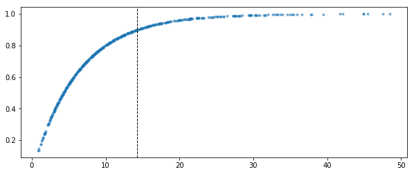
If the player’s NPTwAO/G is equal to the league average, the weight comes out to 0.90, which is the dotted vertical line. High above the average and the score will barely change as the weight get closer to 1, way below and it is affected significantly.

Results

Now let’s look at our new updated rankings.

df['Eff_Factor'] = (df['IOEwAO'] / ppp)
df['Pos_Weight'] =  (1 - 5 ** (-1*df['NPTwAO/G'] / npt_avg))
df['Score'] = df['PGen/G'] ** df['Eff_Factor'] * df['Pos_Weight']


df[['PLAYER_NAME', 'TEAM_ABBREVIATION', 'NPTwAO/G', 'PGen/G', 'IOEwAO', 'Eff_Factor', 'Pos_Weight', 'Score']].to_csv('player_score_results.csv')

df[['PLAYER_NAME', 'TEAM_ABBREVIATION', 'NPTwAO/G', 'PGen/G', 'IOEwAO', 'Eff_Factor', 'Pos_Weight', 'Score']].sort_values('Score', ascending = False).head(25)

	PLAYER_NAME	TEAM_ABBREVIATION	NPTwAO/G	PGen/G	IOEwAO	Eff_Factor	Pos_Weight	Score
90	Damian Lillard	POR	42.07	52.270929	1.261881	1.160534	0.991203	97.782672
215	James Harden	HOU	47.50	56.209223	1.200825	1.104382	0.995224	85.187778
312	Kyrie Irving	BKN	37.89	46.461379	1.254221	1.153490	0.985920	82.568697
383	Nikola Jokic	DEN	29.51	38.220744	1.324564	1.218183	0.963854	81.571881
325	Luka Doncic	DAL	45.48	53.628274	1.196849	1.100726	0.994006	79.611701
319	LeBron James	LAL	44.95	52.825918	1.196271	1.100194	0.993638	78.107706
281	Karl-Anthony Towns	MIN	29.36	37.659113	1.309635	1.204453	0.963238	76.171910
175	Giannis Antetokounmpo	MIL	37.82	45.957049	1.225386	1.126971	0.985809	73.657125
474	Trae Young	ATL	48.45	55.033549	1.158617	1.065564	0.995709	71.265972
133	Domantas Sabonis	IND	24.42	31.984065	1.329774	1.222974	0.935912	64.823166
33	Ben Simmons	PHI	32.90	39.960157	1.235801	1.136548	0.975316	64.486989
42	Bradley Beal	WAS	41.69	47.880432	1.169778	1.075828	0.990818	63.614334
245	John Collins	ATL	18.46	26.192835	1.426170	1.311629	0.874687	63.384272
23	Anthony Davis	LAL	28.05	35.397849	1.273747	1.171447	0.957401	62.465277
424	Rudy Gobert	UTA	12.11	19.491754	1.621689	1.491445	0.743980	62.416989
125	Devin Booker	PHX	39.49	45.710849	1.177698	1.083113	0.988240	62.065480
444	Stephen Curry	GSW	35.49	41.270000	1.210690	1.113454	0.981556	61.780342
239	Jimmy Butler	MIA	30.16	36.820908	1.253294	1.152637	0.966403	61.701542
110	DeMar DeRozan	SAS	31.95	38.943015	1.230290	1.131480	0.972531	61.297541
282	Kawhi Leonard	LAC	35.24	41.560621	1.199544	1.103204	0.981029	59.898776
310	Kyle Lowry	TOR	33.65	39.849228	1.212036	1.114692	0.977313	59.430490
31	Bam Adebayo	MIA	23.29	30.257050	1.319444	1.213474	0.927224	58.093709
73	Chris Paul	OKC	30.27	36.582512	1.232470	1.133485	0.966816	57.186114
76	Clint Capela	ATL	11.53	18.265734	1.608916	1.479697	0.726716	53.481766
221	Jarrett Allen	BKN	9.21	15.802198	1.734327	1.595036	0.645207	52.686162

Based on our new offensive score metric, these were the top 25 offensive players of the 2019-20 season. Note that a few of these players, like Steph Curry and Kyrie Irving missed a lot of games but had high scores the games they did play. Outside of that, I would say this is a pretty reasonable list, to make it to the top you need both volume and efficiency. I also believe playmaking is better rated in this metric than others by including assist opportunities, 2nd assists, and free throw assists.

What I like most about this metric is that volume at the cost of efficiency will hurt your score. For example, lets take an estimated Damian Lillard game where he has 42 NPTwAO and 52 PGen. Now let’s say he continues to take 5 more shots, and makes 2 of them shooting 40% for 4 points, only producing .8 ppp. He would now have 47 NPTwAO and 56 PGen. Let’s look at the difference in final scores between the two instances of the game.

score = 52 ** ((52/42)/ppp) * (1 - 5 ** (-1*42 / npt_avg))
print('Score before shots', score)
score_final = 56 ** ((56/47)/ppp) * (1 - 5 ** (-1*47 / npt_avg))
print('Score after shots', score_final)

Score before shots 89.14031151364419
Score after shots 81.93279421061916

One flaw I have with PER, whose formula can be found here, is that a player can improve their score with volume as long as they are shooting above 30.4% from the field. If I had a player shooting around 35%, I would not want him to increase his volume. My metric makes it so increasing volume is curved by the efficiency factor heavily so that volume is only good when they are producing above league average efficiency.

Flaws

Now I will admit there are some flaws to this metric. Being a purely offensive stat focused metric, it leaves out stats like defensive rebounds, blocks, and steals which could lead to offensive possessions and may unfairly omit a good defender’s actual contribution. It doesn’t adjust for pace so plyers on teams that play faster might get more opportunities to generate points leading to higher scores. Using assist opportunities puts reliance on teammates to make shots, so a player’s playmaking score might be a lot lower on a bad team than it would a good team, as you probably noticed there are only a few instances of a player on a bad team. I didn’t really know how to go about this because leaving out unconverted opportunities misconstrues that player’s usage, but if I were to try and regularize the conversion of assist opportunities it may unfairly punish those who set up their teammates better which is why their team is better in the first place.

This isn’t really a flaw in the stat but another issue is that 2nd assists, free throw assists, and assist opportunities only go back to the 13-14 season when player tracking started so we will be unable to compare offensive scores historically unfortunately, unless we figure out a way to estimate these stats.

Conclusion

I feel this is a good metric to compare offensive performances. This is not to show how skilled a player is necessarily as a lot of it is based on opportunity, but all the time we spend on comparing performance, I think this metric does a better job than most when it comes to offense. It can be used for single game matchups as well as whole seasons differentiating itself to metrics like offensive win shares, and in my opinion pretty unbiased to position.

While there are some flaws and can get a bit complicated, I believe this is a simpler metric to understand than other popular ones that get even more complicated, as it can be boiled down to pretty much volume affected by efficiency. A future task would be to figure out how to incorporate defense which can be extremely hard to measure in numbers.